Contributors:

Balakumar Sundaralingam, Vairavan Sivaraman.

Introduction & Motivation

Predicting an object’s next state without explicitly knowing the dynamics of the object is an interesting problem which would reduce the need for building a physical model of an object. This is even more important in the open world where an object’s dynamics is too complex to mathematically model. Instead of depending on mathematical models, the easier way would be to interact with the object at different contact points and build a classifier to predict the object’s next state. This idea is explored in this paper with experiments to analyze the feasibility.

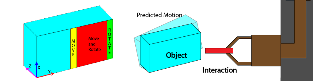
Non-prehensile manipulation also called as graspless manipulation takes advantage of the mechanics of the task to achieve a goal state without grasping, thus simple mechanisms are used to achieve complex tasks. Pushing as shown is a non-prehensile manipulation primitive, where a point or a line contact pushes an object against the friction between the table and object surface. Tumbling is a pushing method in which the object is rotated about an axis around a plane. Pivoting is a method which requires a minimum of two contact points for effective execution. These are some motion primitives in the world of robot object interaction/manipulation of which pushing will be explored to classify the object motions.

Approach

The problem statement here is to predict the labels move and rotate, given a dataset of interactions with the object.

Assumptions

The following assumptions are made about the problem.

1. The object is rigid.

2. The object has only two motion primitives- move and rotate. And it cannot have both the motions at the same time.

3. The contact point force is constant and acts normal to surface of the object.

4. The Object has uniform density,

5. The table surface has an uniform friction coefficient.

Initial Conception

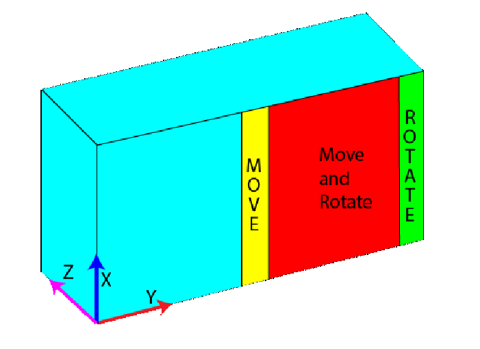
Initially, we attempted to classify a continuous system as in classify if the object is

1. Moving only(Contact is at the centre of the object.)

2. Rotating only(Contact is at the edge of the object.)

3. Moving and Rotating.(Contact is anywhere between the centre and edge of the object.)

Accuracy of Prediction for coupled motions.

Feature Space	Move & Rotate Label Accuracy
	K-NN(K=9)	A-M-Perceptron
Contact Point	38.3%	36.5%
Contact point & Object Pose	48.5%	35.71%

and the predictions for moving and rotating condition were bad as seen in Tab. [table:both] and this was reasoned to be because of learning the weight vector for moving and rotating independently and hence the lack of coupling between the two labels during the learning phase arises. So we focused the project on learning a classifier for moving and rotating independently and removed the motion which had both moving and rotating. The problem is even simpler now.

Problem Statement

Given a dataset $S$ which has the following elements:$x,y,z$ -contact location of the point contact on the object,$\dot{X},\dot{Y},\dot{Z}$ - linear velocities of the object on perturbation, $\dot{\theta}_X$, $\dot{\theta}_Y$, $\dot{\theta}_Z$- angular velocity of the object on perturbation and labels Move,Rotate. This dataset is split in the ratio 8:2 and stored in S_train and S_test respectively. S_train is the training data on which a classifier will be learnt and the prediction accuracy will be checked with S_test. The goal is to obtain a good classifier for the object.

Algorithms/ Classifiers

This problem is a multi label classifier and one way to learn a classifier is to learn the two labels separately and at prediction time, use the two learnt methods to predict each label and count success only when both the labels are predicted correctly. Two classifiers- Perceptron and Support Vector Machines are implemented to learn the motions. The aggressive margin version of the Perceptron classifier is used.

Dataset

Data Collection

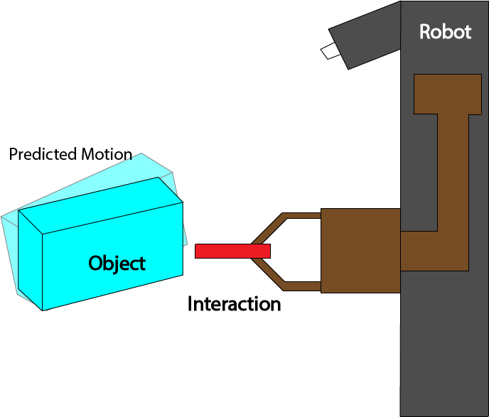
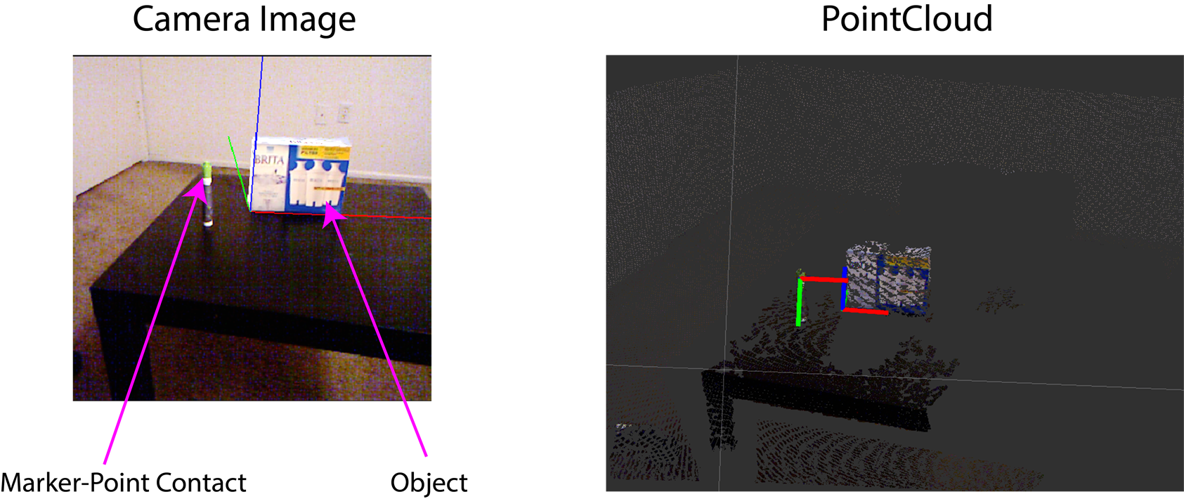
Data was generated from experiments due to unavailability of previous data. The experiment consist of pushing an object(a cuboid) with a marker and recording the change in pose of the object and also the contact point of the marker on the object. The pose of the object and marker is recorded as a time series(useful for velocity calculations). The Kinect sensor is used as the sensor for collecting the pose data. The marker pose is tracked by using simple blob tracking from OpenCV and getting the depth using the pointcloud obtained from Kinect. Tracking the object is complex and thus BLORT tracker. ROS was used as the framework for running the data collection code. The setup is shown below

Data Processing

The training data needed to be labeled and two labels- Move and Rotate were used. Consider an symmetrical object such as a Cuboid. The object will only rotate when the object is pushed from the edge. The object will only move(translate) when the object is pushed at the center. We only assume that there is only two motions available to the object. The data set is manually labeled. The feature space is taken as the contact location(x,y,z) and also the object’s velocity($\dot{X},\dot{Y},\dot{Z}$,$\dot{\theta}_X,\dot{\theta}_Y,\dot{\theta}_Z$). 2000 samples were taken in the dataset, of which 1600 are randomly taken as the training set and the remaining is the test set.

Data Validation

As the data had to manually labeled, the experiments are run separately by first only having the contact point on the center and recording the move-only data and then experiments for rotate-only is performed by having the contact point on the edge.

Feature Space(F-S)

The basic features from data collection was insufficient to learn a good classifier. So to try to improve the accuracy and also to explore how the feature space affects the classification/Prediction accuracy, a number of feature transformations are applied to the dataset. The feature transformations are only done with object data and the contact point data is not modified. The transformations on the object data are based on different norms. A p-norm is calculated as follows: $$ ||\mathbf{x}||_p := \bigg( \sum_{i=1}^n \left| x_i \right| ^p \bigg) ^{1/p} $$ where $x$ is a vector having n components. It can be seen from Eq. [eq:norm] that when p becomes $\infty$, the norm is the largest component of the vector. The object has two velocities-linear($l$) and angular($\omega$) and hence two norms are calculated for the object velocities. The norms are

1. 1-norm of the object velocities($N_1^l$,$N_1^\omega$).

2. 2-norm of the object velocities($N_2^l$,$N_2^\omega$).

3. $\infty$-norm of the object velocities($N^l_\infty$, $N_\infty^\omega$).

With these norms calculated, the feature spaces tested are expanded as follows:

1. $x,y,z,\dot{X},\dot{Y},\dot{Z},\dot{\theta}_X,\dot{\theta}_Y,\dot{\theta}_Z$

2. $\dot{X},\dot{Y},\dot{Z},\dot{\theta}_X,\dot{\theta}_Y,\dot{\theta}_Z$

3. $x,y,z,N_1^l,N_1^\omega$

4. $N_1^l,N_1^\omega$

5. $x,y,z,N_2^l,N_2^\omega$

6. $N_2^l,N_2^\omega$

7. $x,y,z,N_\infty^l,N_\infty^\omega$

8. ${N_\infty}^l$,$N_\infty^\omega$

9. $x,y,z$

With these 9 different feature spaces, the accuracies for each classifier is reported and the results are analyzed in the next section.

Results

The hyper parameters for aggressive margin perceptron(AMP) were calculated by 10 fold cross validation to be $\mu=1$ and similarly for support vector machine(SVM) to be $\rho=1,C=10$. The epoch length was chosen as 100. The result for all the different feature spaces are given in a table below, in which F-S numbers relate to the numbered feature spaces. It is clear that the highest accuracy is shown by svm for F-S 2 which does not have the contact point location as a feature.

Predictions

F-S	Margin-Rotate		Margin-Move		Accuracy%
	AMP	SVM	AMP	SVM	AMP	SVM
1	7.025e-5	0.0036	6.99e-5	0.0037	46.84	51.39
2	1.34e-6	3.82e-8	1.31e-6	3.99e-7	60.7	65.37
3	8.43e-05	0.0037	8.40e-5	0.0036	40.5	51.39
4	0.00065	2.89e-5	0.00065	2.89e-5	37.13	51.39
5	5.35e-6	0.0037	6.1e-6	0.0037	37.75	51.39
6	1.74e-7	1.86e-5	1.74e-7	1.86e-5	37.13	51.39
7	1.012e-5	0.0037	1.01e-5	0.0037	38.67	51.39
8	6.55e-6	1.63e-5	6.60e-6	1.63e-5	37.13	51.39
9	1.91e-6	0.0037	1.91e-6	0.0037	43.6	51.39

Effect of Contact point

The contact point has a negative impact in the results as seen in F-S 2 where the contact point location is not considered and it the best possible accuracy in this project. While in rest of the feature spaces, the contact point is not having a considerable impact. When only the contact points were considered as in F-S 9, it resulted in a low accuracy.

Analyzing the weight vectors

Separate weight vectors were calculated for move and rotate, the magnitude of all the corresponding elements in both vectors were same but the sign of each corresponding element were opposite. So as an experiment, at the prediction state, only either one of the weights was tested and the accuracy resulted in the same as accounting for both the weights. This proves the case that the learning either of the motions is an inverse of the other as we did not account for both the motions combined.

Inference on failures

Classifying a linear dataset seems an easy classifying problem while these experiments prove otherwise. A number of factors could be the reason of which some prominent ones are listed.

1. The motions of the object is not purely linear- when the object is perturbed there will be vibrations due to the impulse force which will be recorded by the tracker and it might be very high compared to the normal motion.

2. The object motion might also be not purely rotating or purely moving at any instant and there might be noise.

3. The dataset might not be sufficient.

4. The force applied on the object may not be a contact force as the object was perturbed by a human and using a robot manipulator might produce better results.

Conclusion & Future Work

Although the problem is linearly classifiable, the learning algorithms are not able to learn it. Future work will be on expanding the feature space to forces and also look into using the pointcloud data without any tracking which would add a lot of dimensions to the problem and might also give a solution for coupling multiple motions such as move and rotate at the same time. Also including different motion primitives such as sliding, toppling and check if the states can be classified is an interesting future direction. Also of interest is including the velocity of the point contact and also the angle at which the contact hits the object, as the contact angle will cause an object to behave differently and it might also be non-linear. For a 2000 dataset, the accuracy of 65.37% is a sufficient result.